On how to read crosstabs
How to read crosstabs? Slice after slice… There is a reason why contingency tables, aka cross tables or crosstabs, are perhaps the most important segmentation tool of professional survey analysts.
Read also Professional Analysis of Survey Data
An old saying goes “You cannot swallow an elephant but you can eat it one slice at a time”. Contingency tables are the tool that slices the survey elephant.
Crosstabs allow you to dig deep into survey data in a systematic way, to turn data in information that can ignite the ability to generate insights. Using them correctly, however, requires some experience, and there are several topics to pay attention to.
How to read cross tables
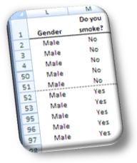
Image 1

Contingency tables are also called cross tables or crosstabs because they actually present the crossed counts of two or more variables.
Counts
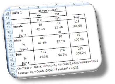
In a two-way cross table two variables, the answers to two questions, are crossed and presented in the form of counts. For instance, we ask 96 men and 129 women whether they smoke or not. The professional cross tabulation of the two variables would look like Image 1, where we read 46 Male respondents said they smoke and 50 don’t while Females smokers to non-smokers are 55 to 74.
Image 2

Read also How to code survey data
Ultimately, cross tables reduce the answers to survey questions to counts. This is the function of contingency tables.
Percentages
Counts are converted to percentages, to help the analyst figure out the proportions between sub-groups of respondents.
Proportions, or percentages, are important because they can lead to identifying groups or clusters of respondents with common characteristics, they help in prioritizing, and very importantly, percentages allow testing the significance of their differences.
Significance test
Image 3

What does testing the significance of the difference of two proportions mean?
Take table 1, where of the 96 male respondents 47.9% said they smoke and 52.1% said they don’t. One could be tempted to state non-smokers outnumber smokers by 4.2%, but this wouldn’t be true. In fact, we are reading the results of a survey conducted at the 95% confidence level and an error level equal to 6.53%. To confirm the proportion of non-smokers is higher than that of smokers it is necessary to test the significance of the difference between the two proportions (4.2%).
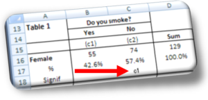
The question becomes: Is the 4.2% difference between smokers and non-smokers large enough to state that the quantity of the latter is really larger than the former? In our case, with a sub-sample of 96 male respondents, the difference is not large enough to confirm the two proportions differ. In this case we must read the percentages as two equal numbers, say 50% and 50%. There is a difference, however, between the proportions of female smokers and non-smokers (see red arrow in Image 3).
MarketingStat’s Insight Discovery Report© applies the Z-Test at the 95% confidence level to verify the significance of differences.
Variables’ dependence and correlation
Sometimes it is useful to know whether the variables of a table are dependent or correlated.
Image 4

Dependent variables are linked by a relationship, and this relationship can be tested with a Chi2 test. The result of the independence test conducted on MarketingStat’s crosstabs is shown under each table and it reads likes this: “Chi² test on table, 95% conf., Ho: col’s & rows indep’t = TRUE”.
If the variables are independent the Chi2 test results FALSE. If they are related the test returns TRUE.
Correlated variables tend to move together. That is, high values of variable A tend to correspond to high or low values of variable B. This is not causation, we cannot say one variable causes the other, but we can still spot dynamics that can lead to concrete actions. For instance:
- Dynamic: The quantity of toothpaste used correlates to smoking habits: Smokers use less.
- Action: Consider educating smokers to use more toothpaste of brand X if the segment is large enough to be financially attractive.
MarketingStat’s tables supply both the Pearson’s Correlation Coefficient and Pearson2 coefficients.
The Pearson Product Moment Correlation Coefficient R is an index ranging from -1.0 to 1.0 and reflects the extent of a linear relationship between two datasets. R, however, does not tell us much about the strength of the relationship between variables, which can be measured with the Coefficient of Determination R2. R2 measures the proportion of variation explained by the independent variable. In the case of Image 2 both values are very low signifying a lack of correlation between gender and smoking habit: “Pearson Corr Coef= -0.041 – Pearson² = 0.002”
Why you should prefer MarketingStat reports
Unlike traditional market research agencies, MarketingStat supplies a complete cross tabulation of the survey questions.
This means all survey questions are cross tabulated with all other survey questions, and percentages are computed in both directions: row and column percentages.
The result is a deck of tables covering every single facet of the survey. And this is not a common report. In fact even major research agencies make only a partial data tabulation using only a few variables, usually between 3 and 5. They claim this is to keep the focus on relevant measures. The truth is that they want to save the time of programming the survey analysis and printing it on paper (traditional agencies still supply clients –and charge for– a paper copy of the tabulation).
CrossTab direction
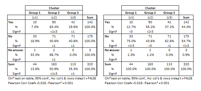
Can you see the difference between these two tables?
Exactly, they show percentages computed in different directions. The table on the left shows row percentages and the other one shows column percentages.
Image 5

MarketingStat makes the value for the client our priority. We provide a complete cross tabulation of the survey questions. No compromise on this.
Need 3-way cross tables?
No problem, we can do it for you.